freeze_Panes
Protected: Freeze Panes
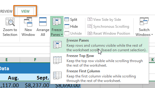
Introduction Whenever you're working with a lot of data, it can be difficult to compare information in your workbook. Fortunately, Excel includes several tools that make it easier to view content from…
Introduction Whenever you're working with a lot of data, it can be difficult to compare information in your workbook. Fortunately, Excel includes several tools that make it easier to view content from…
Working with Rows, Columns and Cells Working with Rows, Columns and Cells In this step by step Excel tutorial, you will learn how to Insert and delete rows, Columns…
Working with Ranges in MS Excel Working with Ranges in MS Excel The term Range is used in MS Excel for the selection of one or more than one cell…
Workbook in MS Excel Workbook in MS Excel: How to Create, Open and Save workbook in Excel Workbook in MS Excel Workbook is considered as an Accounting or calculations…
Ribbon in MS Excel In Microsoft Office 2007, Microsoft introduced “Familiar User Interface” or “Familiar UI”, that replaced the traditional Menu bars and adjustable toolbars with a solitary…
Worksheet in Excel Worksheet in Excel: How to Select, Insert, Rename, Move, Copy and Delete Worksheet in Excel Worksheet in Excel Worksheet is the sub part of a Workbook.…
Important Terminologies in Microsoft Excel Important Terminologies in Microsoft Excel Here you will find important terminologies that are used in Microsoft Excel. MS Excel is widely used all…
Cell References in Excel Cell references are very important in MS Excel. Cell referencing works in formulas and other automations performed within MS Excel. It is further…
Cell References in Excel Cell References in Excel Cell references are very important in MS Excel. Cell referencing works in formulas and other automations performed within MS…