Cell references are very important in MS Excel. Cell referencing works in formulas and other automations performed within MS Excel. It is further classified into different type like relative, absolute and mixed references, and it is very important to understand their difference and purposes.

Relative Reference

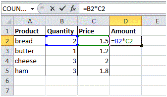
By default, MS Excel uses relative reference. The formula shown in Cell D2 in the figure below. In this formula, Cell D2 references to Cell B2 and Cell C2. Both references are relative as they both are coming in a sequential manner

Let’s further observe it simply filling the formula from D2 to D5. You can do this in multiple manners as discussed in earlier tutorials like using Copy and Paste feature or Formula Fill feature.

Now, in this addition, Cell D3 is referencing Cell B3 and Cell C3. Cell D4 is referencing Cell B4 and Cell C4 and finally, Cell D5 is referencing with Cell B5 and Cell C5. In simple words: each cell references its two left side neighbors.

Absolute Reference

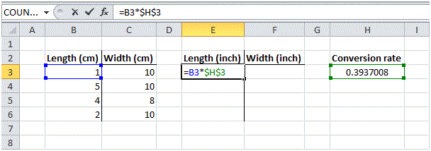
The formula shown in Cell E3 in the figure below is associated with absolute referencing. In this formula, Cell E3 references to Cell B3 and creates an absolute reference with Cell H3. The $ symbol represents the absolute reference of the cell.

1. To create an absolute reference with cell H3, place a $ symbol next to the column letter and row number of cell H3 (i.e. $H$3) in the formula of cell E3.

2. Now you can quickly fill this formula to the other cells.

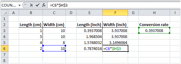
It is evident that the reference to cell H3 is fixed and has not changed by dragging or filling. As a result, the correct lengths and widths in inches are calculated.

Mixed Reference

At times it happens that you need a combination of both relative and absolute references and this termed as Mixed Reference.

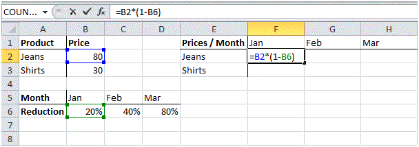
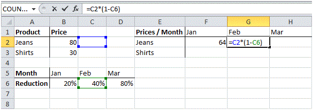
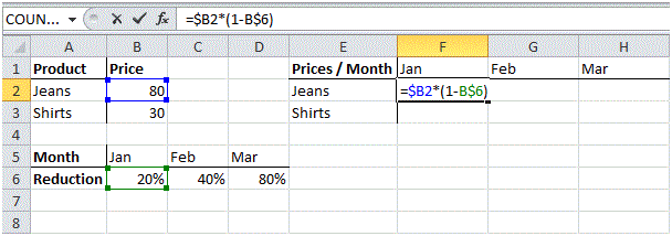
In the formula in cell F2 shown in the figure below, is the example of a Mix Reference.

Now, if you copy this formula to other cells or fill it. Drag cell F2 across one cell, and look at the formula in cell G2.

Well, the reference of the price should have been fixed to column B. The issue is that the formula is missing the $ symbol as described in the previous section.

Now, after putting the $ sign before Column Reference B, lets repeat the previous step again

Now, quickly drag this formula to the other cells.

You will notice that the references to column B and row 6 are fixed.